In Module 2, we learned the core logic of Bayes’ Theorem and applied it to binary problems: Is a diagnosis correct (yes/no)? Is a warranty a good value (yes/no)? This was a great way to learn the formula, but it’s not how we (or our students) usually think about the world. “Yes” or “no” is an overly simplistic view of how our beliefs work. While frequentist null hypothesis tests are focused on a binary outcome, “reject” or “fail to reject,” Bayesian methods often represent an entire distribution of possible outcomes.
Our beliefs are rarely just “on” or “off.” We don’t just ask, “Does this make a difference?” We ask, “How much difference does it make?” We don’t expect a delivery at an exact time, but within a range of possibilities.
This module moves from binary outcomes to distributions of belief. We’ll explore how to represent our uncertainty as a distribution and how that distribution changes as we gather more data. We’ll introduce different types of priors, see how beliefs converge over time, and use interactive examples to understand how continuous data (like time) can update our beliefs moment by moment.
Learning Objectives
Upon completion of this module, you will be able to:
Explain why representing belief as a distribution is more intuitive than a binary outcome.
Differentiate between an informed prior and an uninformed prior.
Describe how different priors converge (or "wash out") as more data is collected.
Define a Probability Density Function (PDF) and its role in modeling continuous data (like time).
Analyze how a stream of data updates the relative likelihoods of multiple competing hypotheses.
The World is Full of Variability, So We Are Full of Uncertainty
If the world didn’t vary, you’d know exactly what to expect. But, because the world does vary, you can represent a wide range of values in your mind to capture that variability. You can even think of the spread of that distribution as being related to how uncertain you are.
If your beliefs are tightly clustered around a small range of values, you’re probably pretty certain about what to expect. But if your distribution is wide, it suggests you are really not sure what is going to happen and are keeping open to many possible outcomes. Thinking in terms of distributions allows you to shift to a more nuanced question. Instead of “am I hungry?” you can shift to, “How hungry am I?” Editor’s note: I may or may not have been hungry when putting together this module.
A Note on Effect Sizes
If you’re familiar with t-tests and ANOVAs, you probably are aware of the recent emphasis on including effect sizes in statistical reporting. This is the frequentist solution to the “how much difference does it make?” question. It’s worth noting that the need for effect sizes should reinforce the notion that p-values do not provide you with this information. As we noted in module 1, A lower p-value tells you nothing about how strong of an effect was observed. And in our Bayesian t-test module, you’ll see our Bayesian t-test explores effect size directly at the heart of the test.
Food for Thought: Everyday Bayesian Reasoning
There are a zillion everyday examples where we think of ranges rather than binary outcomes. It's probably the rule rather than the exception, but here are a few that come to mind:
Food Delivery: Your expectation for a food delivery isn't a single number, but a distribution of times. An arrival at 15 minutes is surprising, as is an arrival at 90 minutes. Your feeling of surprise changes as time passes, first decreasing as you enter the expected window, then increasing again as the delivery becomes late.
Gas Tank: Your car's gas gauge isn't a binary "gas" or "no gas" state. You have an expectation—a distribution of possibilities—for how far you can drive after the warning light comes on.
"Bottom of the Bag" Fries: When you get fries from a fast food place, you don't expect a specific number of fries left at the bottom of the bag, but a range of possibilities, from a single sad piece to a glorious handful.
4. Priors, Updating, and Convergence
Bayesian methods have the idea of variability “baked in,” and the goal is to have your mental representation match the real world’s distribution of values. As you go through the Bayesian updating process, your beliefs become more and more accurate.
At Six Dudes, they give you way too many fries. OK so it’s AI slop, but let’s consider that the prompting itself might be an art. It was my vision, the AI just helped make it reality. But whatever you do, I do NOT recommend that you zoom in on the guys – er, dudes.
The first time you order from a particular food place with, I don’t know, some number of guys involved– you might not know what to expect. My friend M might keep a broad prior and “wait and see,” but I might base my prior on previous experiences with other restaurants. In either case, once you see how many fries you get, you can update your beliefs accordingly for next time. The more surprising the data, the more your belief shifts. But even though our priors were different and our updated beliefs are different, our beliefs are now much more similar than they were before.
Informed vs. Uninformed Priors
Uninformed priors try to be impartial, whereas informed priors try to incorporate previous knowledge.
Broad priors that are centered on a neutral theoretical value (such as estimated differences of zero) are called “Uninformed Priors.” The idea is to cast a low, wide net such that you aren’t really committed to any particular value, and you are therefore ready for whatever the data throws at you. It’s basically a neutral starting point. Informed priors, on the other hand, may use estimates based on previous knowledge or inferences, but may be more biased from the start.
How long would you wait at a traffic light before deciding that it is broken?
5. An Interactive Example: The Traffic Light
As you exist in the world, you are constantly learning things and representing things in your mind, even if you don’t realize it. For example, if you roll up to a traffic light, how long would you wait at the red light before you would decide the traffic light is broken and just keep driving on?
Every time you’ve waited at a red light in the past, you’ve encoded that into your brain in some form or fashion, I would argue through a Bayesian updating process, to form a representation of the distribution of light times you’ve encountered. Here in San Antonio, the average wait time is between 60 and 90s according to the city.
So for each moment you sit there, what is the probability that the light is broken, given how much time has passed? The applet below allows you to see how your belief changes over time while you wait for it to turn green.
Let’s calculate P(Broken | Time).
Prior P(Broken): It is fairly rare to run across a broken traffic light but it does happen. Let’s say it’s very low, maybe 1 in 1000 (0.001).
Likelihood P(Time | Broken): If the light is broken, the probability of you waiting a long time is high, let’s say 99%.
Marginal Likelihood P(Time): Probabilities of wait times for a normal, working light can be found using the city data (mean = 75s) and an exponential probability distribution. This is a common statistical model for the time between events, and it’s a great fit here because it naturally captures our real-world experience: short waits are very common, and the chances of having an extremely long wait get smaller and smaller as time goes on. The applet uses the Probability Density Function (PDF) from this model as the P(Time) term. The PDF gives us a measure of how relatively likely it is to still be waiting at any specific moment. An observation at a common time (like 10 seconds) has a high density and isn’t surprising, while an observation at a rare time (like 180 seconds) has a very low density, providing strong evidence that something is wrong.
Scenario 1: Waiting for 10 seconds
The probability that you are still waiting after 10s at a normal light is high. The PDF models it at 1.2% which sounds low but in PDF terms is pretty big (see the PDFs content box for more info). We can set P(Time) = 0.012.
P(Broken|10s) = (0.99 * 0.001) / 0.012 = 0.0825. So, belief that the light is broken should be well under 10%.
Scenario 2: Waiting for 3 minutes (180s)
The probability of waiting 3 minutes is very low, say P(Time) = 0.01.
P(Broken|180s) = (0.99 * 0.001) / 0.01 = 0.10. Your belief has shifted significantly to a 10% chance the light is broken.
This process happens automatically in our brains, and differences in priors can explain why some people are more patient than others. Some people may assume it’s malfunctioning and run the light earlier than others.
Try it!
In the applet below, you can adjust the slider and see how the posterior likelihood changes as time passes. Picture yourself sitting at a traffic light while the seconds tick by, and you become more and more convinced that it’s not working properly.
P(Broken|Time): Your updated belief the light is broken.
P(Time|Broken): The likelihood of waiting this long if the light were broken.
P(Broken): Your prior belief that any given light is broken.
P(Time): The probability of waiting this long for a normal light.
10s
Calculating...
Change in Belief Over Time
Probability Density Functions (PDFs)
Getting into PDFs is probably more in-depth than you can go in a short module for an undergraduate course, but it's worth mentioning here. In simple terms, a Probability Density Function (PDF) is a curve that shows you where the outcomes for a continuous variable (like height, weight, or time) are most likely to fall.
The key thing to remember is that for a continuous variable, the probability of getting one exact value is zero. For example, the probability of someone being exactly 6 feet tall (not 6.0001 or 5.9999) is technically zero because there are infinite possible heights. But if you add up every point under the curve, you'll get a value of 1, or 100% probability.
Because of this, a PDF doesn't tell you the probability of a specific outcome. Instead, its height tells you the relative likelihood or density of outcomes in that area. A high peak on the curve means values in that region are very common, while a low, flat part of the curve means values in that region are rare. It also means that even for highly probable events, the probability is very low.
[Calculus has entered the chat...] Yes, to find the area under the curve you've got to use some calculus. But if you didn't take calculus, or your students didn't take calculus, don't worry -- the machine will do all that for us. But if you hear calculus come up, that's the main place in Bayesian stats that it pops up: Calculating an integral from point A to point B.
The Population Density Analogy
A great way to think about a PDF is to imagine a population density map.
The Map is the PDF: The entire map represents all possible outcomes.
The Color is the Density: The color at any single point on the map represents the population density there. A dark red spot over a city like San Antonio has a very high density. A light green spot in a rural area has a very low density.
A Single Point Has No Probability: If you ask, "What's the probability of finding a person at these exact GPS coordinates?" the answer is zero. A single point is too small to contain a person.
Probability is an Area: To find a probability, you have to look at an area. The probability of finding a person within a one-square-mile block of downtown (a high-density area) is much higher than finding a person in a one-square-mile block of ranchland (a low-density area).
This is exactly how a PDF works. The height of the curve (the "density") tells you which regions are more "populated" with likely outcomes. To find an actual probability, you have to calculate the area under the curve for a specific range of outcomes.
6. Comparing Multiple Hypotheses
One strength of a Bayesian approach is that you don’t have to be limited to a single hypothesis; you can hold several at once and compare their likelihoods based on incoming data. We can show this in a simple example by following a sequence of coin flips. Now, I usually try to avoid classic statistical problems like “drawing colored balls from urns” that don’t have much applicability to the real world, but coin flips are a pretty well used source of random data that people are familiar with. But more importantly, we can ask an incredibly practical question: How much do you trust the flipper?
Imagine I offer to flip a coin to decides who buys lunch today. Since that might seem like a weird question out of the blue, maybe you want me to do a few “test flips” before the flip that drains your wallet to fill my stomach. You can think of at least 3 possibilities:
H1: The coin is fair, 50/50 (H/T)
H2: It’s a two-headed coin (H/H)
H3: It’s a two-tailed coin (T/T)
Your prior could be informed by things like how often people ask you to do coin flips, your past history with trick coins, or your past history with me in which I have established myself as “a lil’ stinker.” Let’s assume for now your prior for each hypothesis is equal and see how the likelihoods change as we collect data.
Flip 1: Heads. H1 and H2 get stronger. H3’s likelihood dramatically decreases, since you can’t get heads with a two-tailed coin. Any further heads flipped will reinforce this belief. So, on this first flip we can readjust our beliefs in these 3 possibilities, and carry our new priors forward to the 2nd flip.
Flip 2: Heads. H1 and H2 both get stronger. But notice that the probability of flipping heads is higher for H2 than H1, so while both are plausible given two heads flipped in a row, the evidence is more consistent with H2 so it will be relatively stronger.
Flip 3: Heads. H1 and H2 both get stronger, but H2 is gaining much more strength relative to H1 now. While the probability of flipping heads 3 times in a row is about 1 in 8, which far from impossible, are you willing to stake lunch on this coin at this point?
Hopefully that journey helped show you what it feels like as we update the likelihoods of different hypotheses as a stream of data comes in, where their relative likelihoods shift your beliefs.
The Bayesian Way: Testing for every possible outcome
If we want to formalize this, we can actually compare the likelihoods of a series of flips for not just one hypothesis, or three, but we can compare the likelihoods of every possible coin outcome, from all tails (0) to all heads (1). This gives us a whole distribution of likelihoods for the coin (see the Coin Flip applet’s top graph). As we gather data by flipping coins, the likelihoods for each of these outcomes shift.
This likelihood distribution can then be combined with our prior distribution by multiplying point-by-point for each possible coin fairness outcome. Multiplying entire distributions can be computationally complex, but we have computers for that. Now, as you can imagine, multiplying small numbers by small numbers gets you some extremely small values, and any areas under curves that used to add up to 1 no longer do. But that’s the real value of the marginal likelihood function: By dividing by the marginal likelihood, everything rescales back into more reasonable numbers, and the result is your updated posterior distribution. You can see this in action in the coin flip applet.
Bayesian Coin Flip Explorer
See how Likelihood and a Prior belief combine to form a Posterior belief.
Heads
0
Tails
0
MLE (θ)
N/A
Current Sequence
No flips yet.
1. Likelihood Function
How well does each possible coin bias explain the data you've seen?
2. Posterior Distribution
Your updated belief, combining the Likelihood with a Prior belief that the coin is fair.
Things to Try
1. The Power of Evidence: The prior believes the coin is fair. Enter a sequence of five heads (HHHHH) to see how quickly strong, consistent evidence can pull the posterior belief away from the prior.
2. The Stubborn Prior: With only a small amount of data, the prior has a lot of influence. Enter a short, balanced sequence like (HT). Notice how the posterior distribution barely moves from the prior's initial position.
3. Confirming Your Beliefs: What happens when the data matches your prior? Enter a long, balanced sequence like (HTHTHTHTHT). Watch as the posterior becomes sharper and more confident, centering right over the prior's peak at 0.5.
Module Summary
Congratulations! If you made it this far, you’ve got the basics down. You now know:
The four parts of Bayes theorem: The posterior, the prior, the likelihood, and the marginal likelihood (base rate). Solving Bayes’ equation helps us update our beliefs on the basis of new evidence.
The difference between likelihoods and probabilities. Likelihoods describe how well the hypothesis fits the data, whereas probabilities describe how well the data fits the hypothesis.
We went through several different binary examples, to show how this can apply across different situations
Different priors lead to different outcomes, but tend to converge on the same answer over time (i.e., they “wash out”).
You can use a more neutral “uninformed” prior, or an “informed” prior based on what you already know.
You can see how much difference your prior makes with a robustness check which tests several priors at different extremes.
You can apply these concepts not just to binary outcomes, but also distributions of belief.
Surprising data shifts your beliefs more.
Probability Density Functions (PDFs) are a key tool for Bayesian analysis, even if (like me) you prefer to let the computer do the calculus for you.
Bayesian methods can compare several hypotheses at once and compare their relative likelihoods.
Key Terms
Bayes’ Theorem: A mathematical formula for calculating conditional probability, used to update beliefs in light of new evidence. P(H|D) = P(D|H) * P(H) / P(D).
Prior Probability (Prior): An initial belief about the probability of a hypothesis being true, before considering the current data.
Likelihood: The probability of observing the data, given that the hypothesis is true. It connects the data to the hypothesis.
Posterior Probability (Posterior): The updated belief in the probability of a hypothesis being true after taking the data into account.
Marginal Likelihood (Evidence): The total probability of observing the data, calculated across all possible hypotheses. It acts as a normalization constant.
Bayesian Updating: The process of revising a prior belief into a posterior belief after observing new data.
Distribution of Belief: The representation of a belief as a range of possible values with varying probabilities, rather than a single point estimate or a binary outcome.
A Note on Your Teaching Journey
As instructors, we are lifelong learners. It's perfectly okay – and often incredibly empowering for students – to share your own learning journey. You might say something like:
"I wasn't taught these concepts when I was a student, but I believe they're incredibly valuable. We're going to explore them together, and I'm excited for us to learn this powerful new way of thinking."
Your authenticity will foster an engaging and open learning environment.
What’s next:
In the next module, you’ll learn how to conduct an equivalent of a Bayesian t-test using the free software JASP and interpret the results. If you prefer to use R or python, I will provide some resources to help you get started on that, too – but JASP has a very user-friendly interface and a quick learning curve, so I’ve chosen it for this demo.
 At Six Dudes, they give you way too many fries. OK so it’s AI slop, but let’s consider that the prompting itself might be an art. It was my vision, the AI just helped make it reality. But whatever you do, I do NOT recommend that you zoom in on the guys – er, dudes.
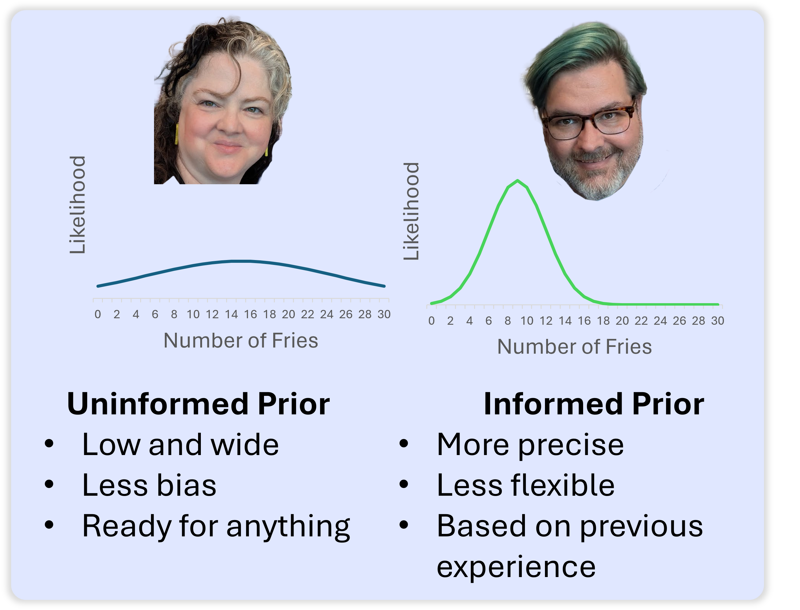
How long would you wait at a traffic light before deciding that it is broken?